I. The End-to-End Large Model Business Workflow

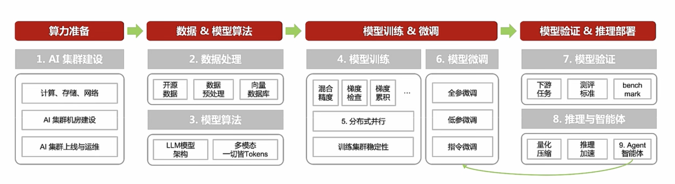
1. Building AI Clusters: Computing, Communications, and Storage Infrastructure

2. Large Model Data: Datasets, Data Processing, and Vector Databases

3. Large Model Algorithms: From Traditional NLP to Pretrained LLMs

4. Large Model Training: Common Algorithmic Approaches and Stability Analysis

5. Distributed parallelism: model parallelism, data parallelism, optimizer parallelism, etc.

6. Large Model Fine-Tuning: Full-Parameter, Parameter-Efficient, and Instruction Fine-Tuning Algorithms

7. Large-model inference: quantization and compression, inference with extended sequence lengths, caching methods

8. Large Model Evaluation: NLP Downstream Tasks, CV Downstream Tasks, and Evaluation Plans

9. Large language model agents: the RLHF process, agents, lifelong learning

II. Vectors

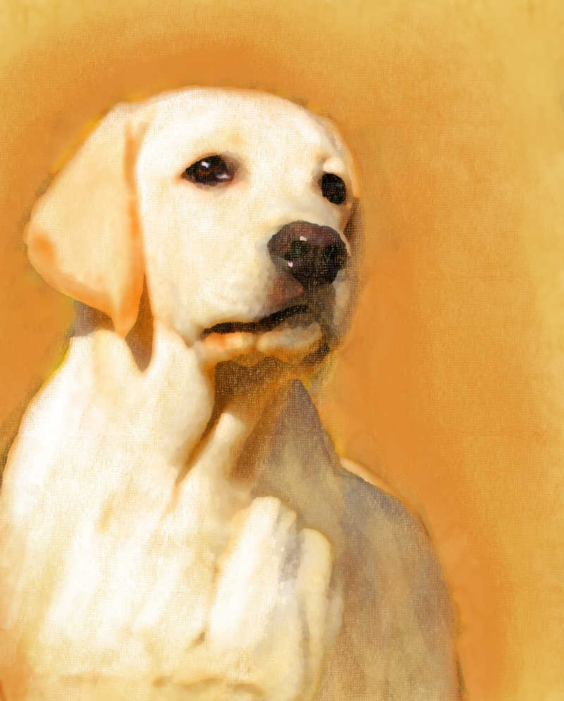
People familiar with dogs can quickly distinguish their breeds. They can do this because they observe the dogs' characteristics from different perspectives, such as body size.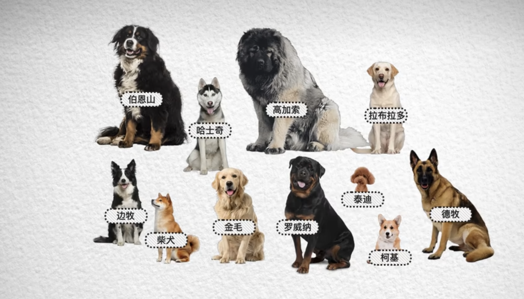
If we use a coordinate axis to represent their size, these dogs will fall at different positions along it. However, relying solely on size is not enough, as some of them are very similar in size.
Next, we examine another feature, such as fur length, and create another coordinate axis. This lets us distinguish some dogs that share the same size characteristics
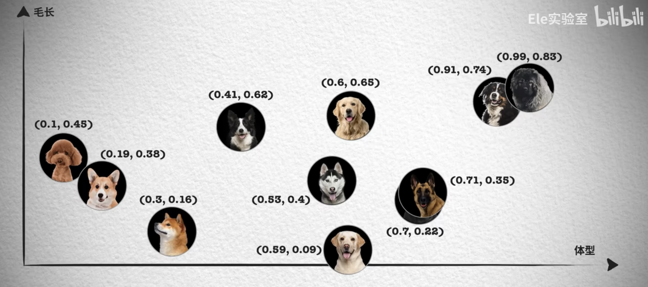But some still overlap, so we need to continue observing from more perspectives, such as the length of the nose.
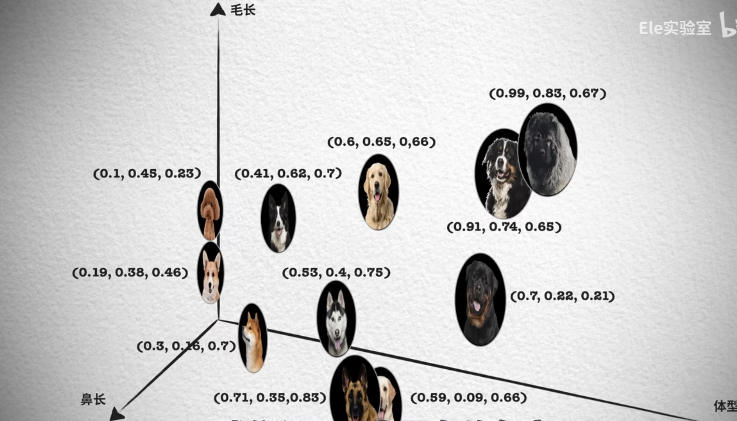We can add more dimensions, such as eye size. We cannot plot in four-dimensional space, but it is easy to represent this numerically in the coordinates: just keep appending values.
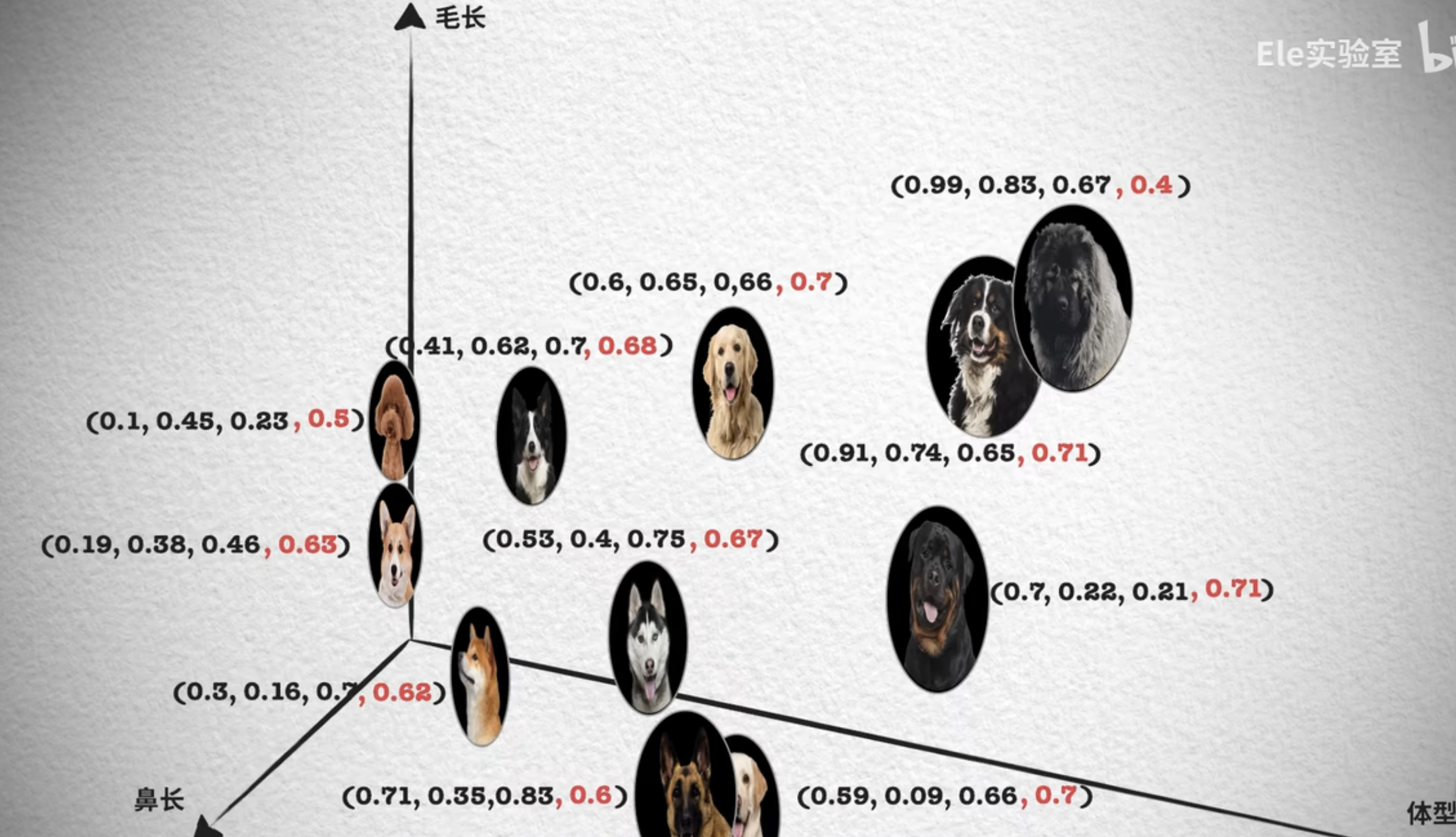We can also examine a dog’s characteristics from more perspectives, or dimensions, such as leg thickness, how curly its fur is, or even abstract aspects such as obedience and usefulness as a working animal. The more dimensions we use, the better we can distinguish between dogs. At the same time, the space containing the coordinate points also has more dimensions.
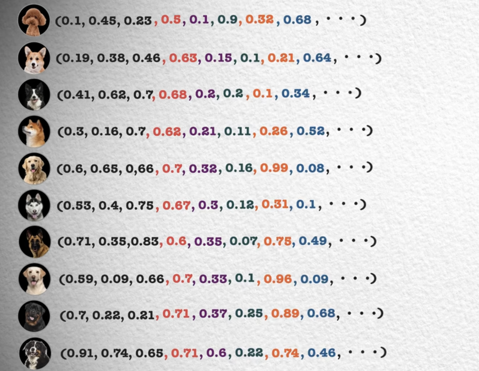In fact, almost anything, beyond just dogs, can be represented this way. It can be something concrete, or abstract emotions such as joy, anger, sorrow, and happiness, or partings and reunions. Different things have different manifestations, or different numerical values, across different feature dimensions, so each ultimately corresponds to a coordinate point in a high-dimensional feature space. Within these broader scopes, however, we may need more feature dimensions to distinguish things well. Perhaps hundreds or thousands, or even tens of thousands.
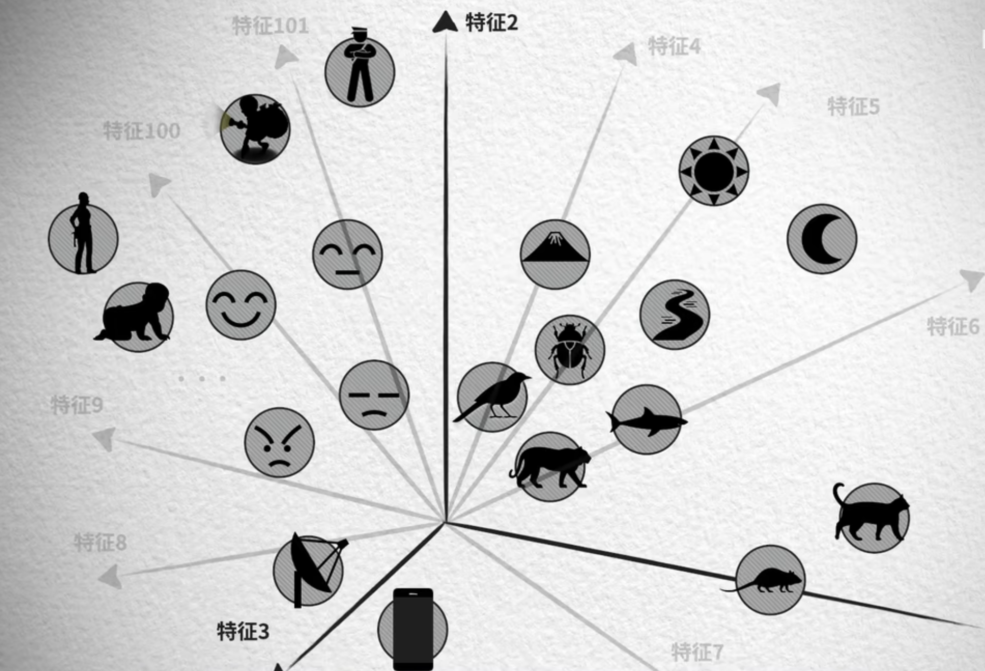However, since we cannot draw diagrams in more than three dimensions, we will explain using two-dimensional coordinates.
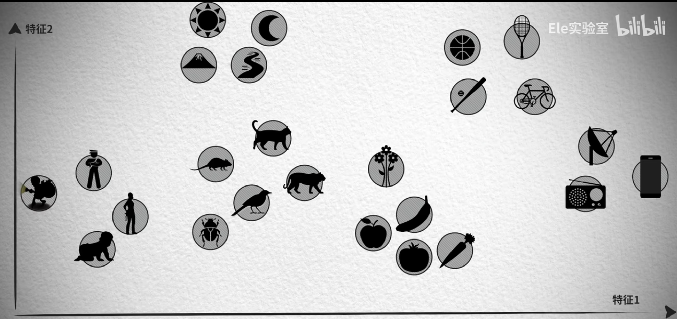We will find that points closer in meaning cluster more tightly in space, while points with very different meanings lie far apart. Taking this a step further, if we use the coordinate origin as the starting point and these coordinate points as the endpoints, we obtain vectors with direction and magnitude.

If images are converted into vectors, searching for similar vectors enables image-based image search
If videos are converted into vectors, similar videos can be recommended by searching for similar vectors
If products are represented as vectors, similar vectors can be searched to recommend related products based on the product the user is currently viewing
By converting text into vectors, an intelligent question-answering system can find previously resolved questions similar to the user's current question for reference

III. Vector Databases

With the arrival of AI, vectors will become an important form of data. Traditional databases are not suitable for storing and retrieving vector data, so a purpose-built database is needed to address these issues. This may become part of the data infrastructure of the future. Unlike traditional databases, which store data tables and use query statements for precise searches, vector databases store vector data, and their queries search the database for vectors most similar to the query vector, making the process somewhat approximate.

1、Vector queries

One major use case for vector data is to find the most similar vectors among a large collection, given a query vector. This is known as the nearest-neighbor problem, and algorithms that accomplish this are called nearest-neighbor algorithms. One of the most immediately obvious approaches is brute-force search: compare every vector's similarity to the query vector in turn, then select the few with the highest similarity. There are many specific ways to compare the similarity of two vectors,Euclidean distance and cosine similarity.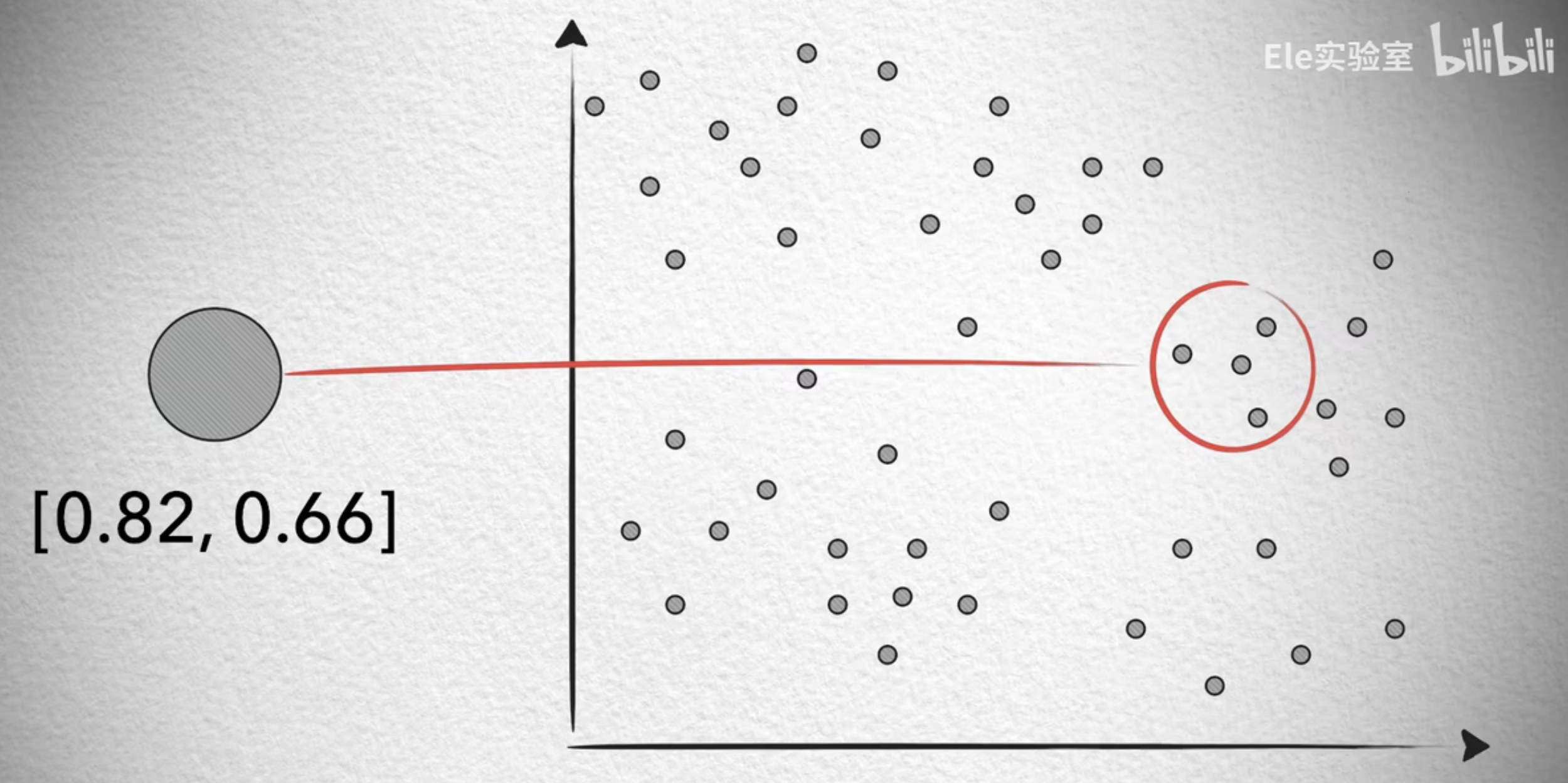

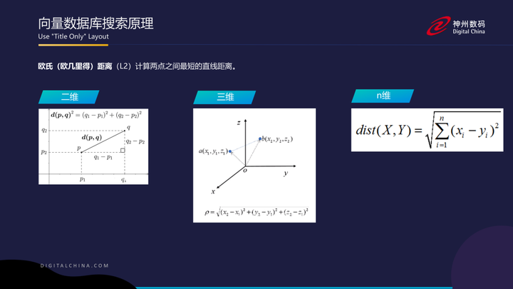
• Euclidean distance is the straight-line distance between two vectors. In a two-dimensional coordinate system, given two vectors p and q, the Euclidean distance is the length of the straight line connecting p and q. In a three-dimensional coordinate system, each vector contains three coordinates, x, y, and z, and the distance between any two points is calculated using the formula. In an n-dimensional coordinate system, there are 100 coordinates, and the distance between any two points is calculated using the formula. The shorter the distance, the greater the similarity between the two vectors in certain dimensions
  
  

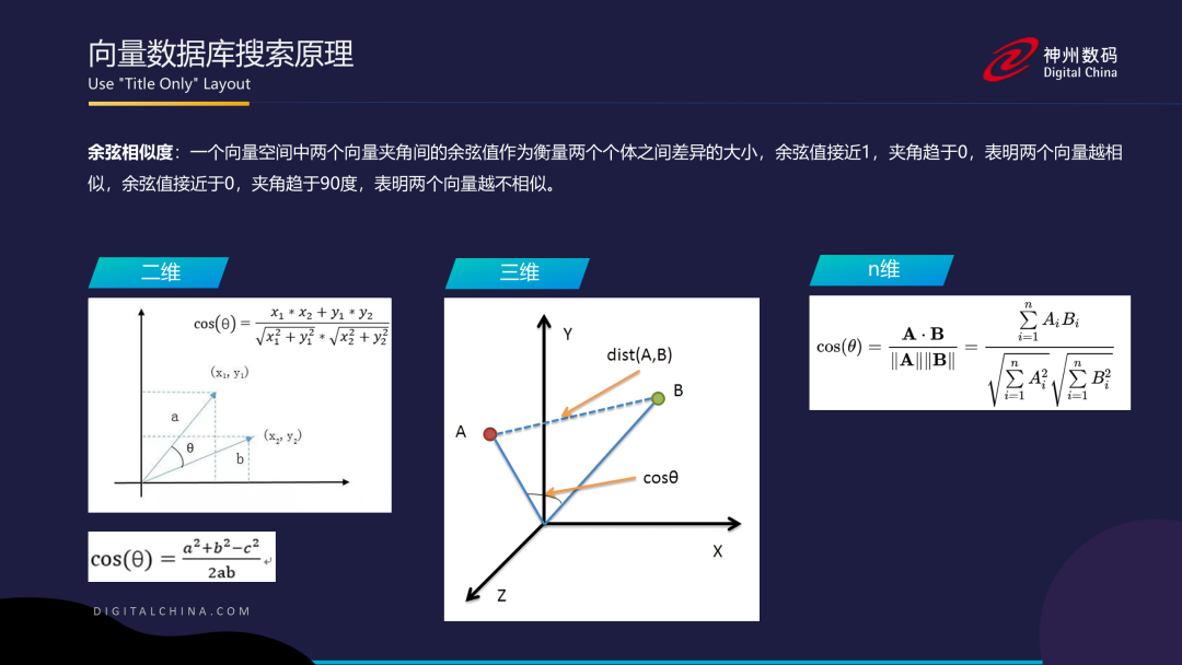
• Another approach is cosine similarity. Besides distance, we can describe the relationship between vectors using the angle between them. In a two-dimensional coordinate system, a smaller angle indicates a stronger relationship between two vectors. We can use a formula to calculate the cosine similarity between any two vectors. The same principle can also be used in a three-dimensional coordinate system to calculate the angle and cosine similarity between any two vectors.
  
  If there is too much vector data, this unsophisticated brute-force method will result in extremely long search times. Its search quality is indeed perfect, however, because it really does compare every vector. If the database is relatively small and the time needed to traverse all vectors is acceptable, this can be a good method. In real-world applications, however, datasets are usually fairly large, so ways to optimize the search must be found.

2、Vector indexes

The principles of vector database retrieval were explained earlier, but in practice, similarity matching in a vector database cannot rely entirely on direct formula calculations, because vector databases usually contain large amounts of highly dimensional data. Using a formula to calculate the similarity between two 1000-dimensional vectors requires considerable computation and places heavy compute-intensive demands on the CPU. With a hundred million vectors, calculating the similarity for each one would incur even greater time and computational costs. This brings us to a concept called a vector index.
A vector index is similar to an index in a relational database, with one difference. In a vector database, a vector index returns approximate results, rather than results that are 100% accurate.A vector index describes how high or low the degree of similarity is. We therefore call it approximate nearest neighbor search (ANS). Without a vector index, searching for similarity to a vector is like a full table scan in a relational database. However, it requires an additional layer of computation on top of the full table scan, making it much more costly than a full table scan in a relational database.
Based on their implementation, ANNS vector indexes can be divided into four major categories:

• Tree-Based Indexes

• Graph-Based Indexing

• Hash-based indexes

• Quantization-based indexes

1、Tree-based methods

The main idea behind tree-based methods is to partition data, much like a binary search tree, reducing the search space during searches to enable fast retrieval. However, this approach is unsuitable for high-dimensional spaces. The main tree-based methods include KDTree (K-Dimensional Tree) and Annoy (Approximate Nearest Neighbors Oh Yeah).
1.1 KDTree
KDTree construction is likewise based on recursive partitioning. First, select the dimension with the greatest variance and use the median of all data along that dimension as the split point to divide the hyperrectangular region into two subregions. Values below the median go to the left, and values below the median go to the right. Recursively construct the left and right subtrees until all the data has been partitioned.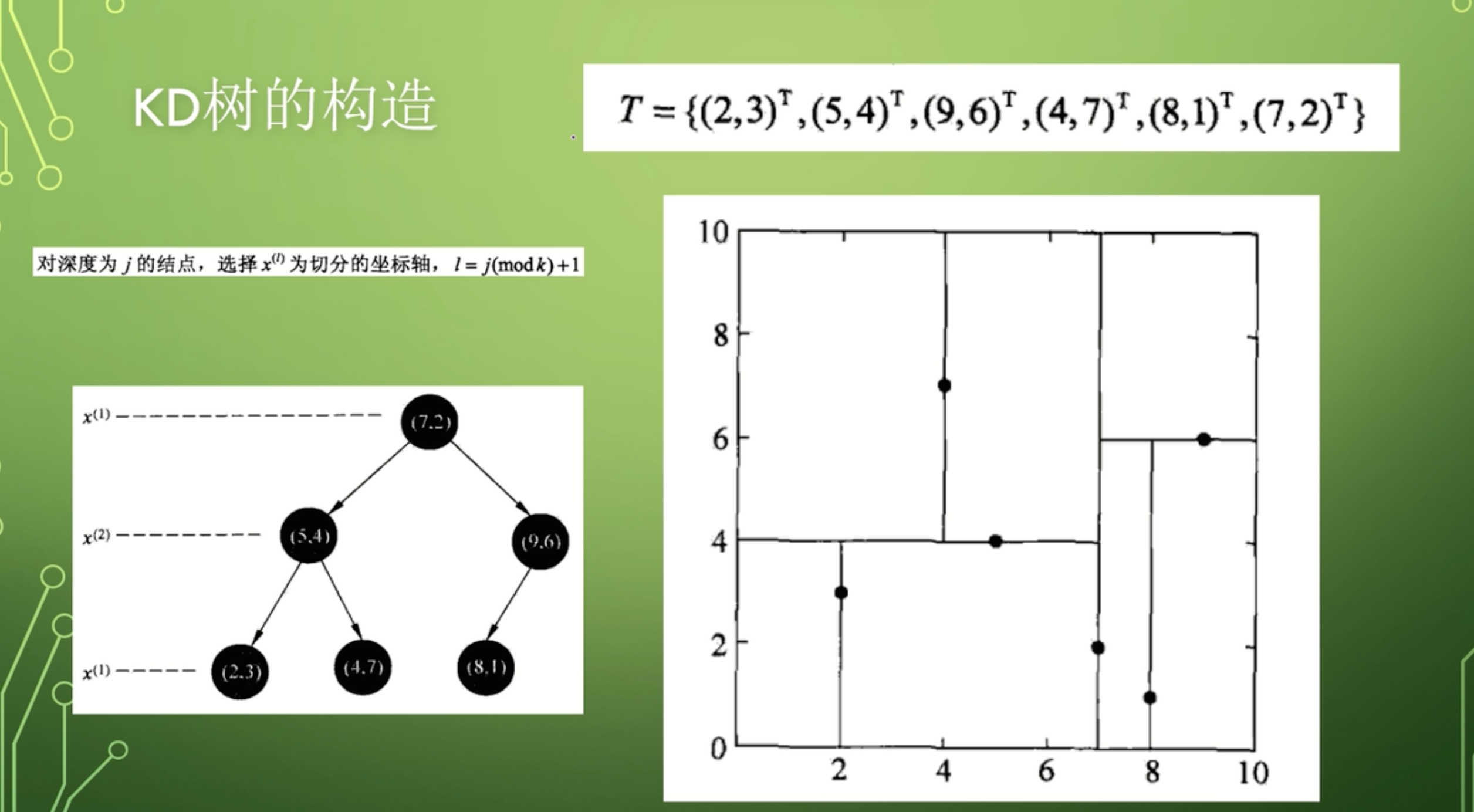

KDTree-based search procedure:
1, For query point p and the current node's splitting dimension d, compare p's coordinate in dimension d with the node's value; if it is greater, go to the left child; if smaller, go to the right child;
2、Continue traversing until reaching a leaf node, mark it as visited, and calculate the distance to the leaf node as the nearest distance;
3, Backtrack from the leaf node, checking at each step the distance between p and the unvisited branch of the parent node.
a) If the distance between this branch node and p is greater than the current nearest distance, continue backtracking upward until reaching the root node;
b)If the distance between this branch node and p is less than the current nearest distance, use this branch and follow step 1 and step 2 until reaching a leaf node, then update the nearest distance between the leaf and Q.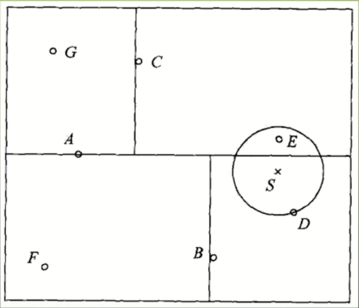

1.2Annoy
Annoy uses hyperplanes to partition the space. It uses KMeans(k=2) to find two cluster centers, then takes the plane perpendicular to the line connecting the centers as the partitioning hyperplane, repeatedly iterating until the number of data points in each subspace falls below a specified threshold.
 

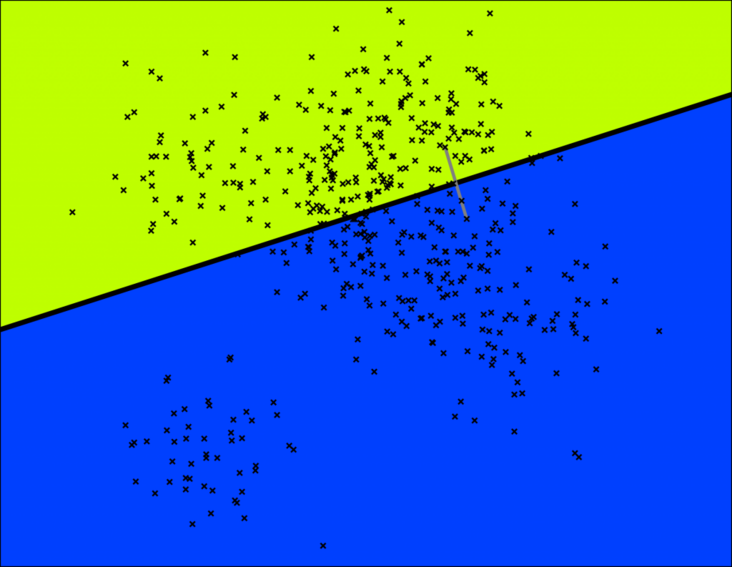
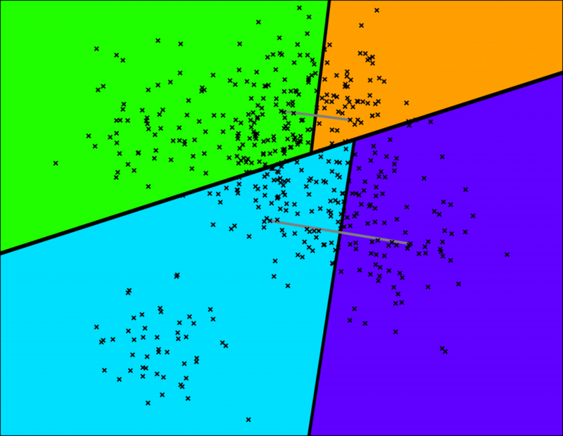
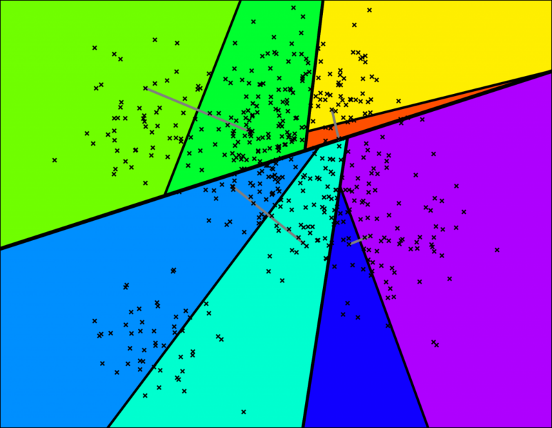
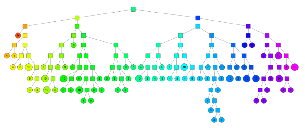
To search for any point in this space, you can traverse the binary tree starting at the root. Each intermediate node (the small squares in the tree above) defines a hyperplane, which lets you determine whether to continue to the left or right child node. Searching for a point can be completed in logarithmic time, corresponding to the height of the tree.

Advantage: Higher accuracy for lower-dimensional data Disadvantage: Cannot fully capture data complexity, with lower accuracy for high-dimensional data

2、Graph-Based Methods

Graph-based methods primarily use the graph data structure, exploiting connectivity between neighboring nodes to build highways and turn the problem into graph traversal. This quickly narrows the search scope and speeds up retrieval. However, graphs are relatively complex data structures. To achieve the fastest possible retrieval, the entire graph is generally loaded into memory, resulting in very high memory usage, but fast retrieval and high recall.

The main graph search algorithm commonly used today is HNSW (Hierarchical Navigating Small World), while NSW (Navigating Small World) is its predecessor and is also worth understanding.
2.1 NSW
NSW adds the following rules to naive graph construction: every node must have neighboring nodes; neighboring nodes must be connected by edges; and the number of neighbors is a hyperparameter specified by the user. It is mainly intended to address some limitations of naive graph construction.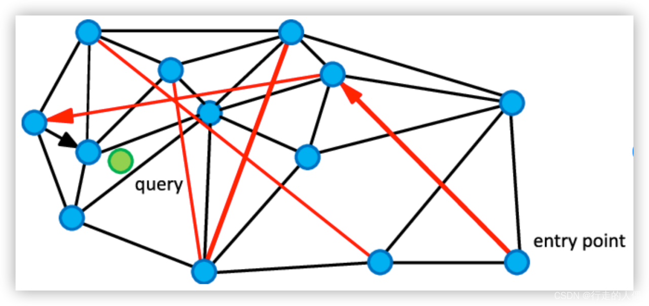
NSW graph construction process:
When inserting a new node, first find the m nodes closest to it, then connect the new node to those m nodes.
NSW search process：
For query data q, randomly select an entry point node and its neighboring nodes from the graph, and calculate the distances from the entry point and its neighbors to p. If a neighbor is closer to p than the entry point is, designate the closest node and continue until finally finding a point whose neighbors are all farther from the query than that point is.
As shown above, to find the nodes closest to the green query node in the constructed nearest-neighbor graph, begin at randomly selected entry points. First, the red long-links quickly lead to nodes near the query, then the black short-links lead to suitable points.
NSW is also an approximate computation and cannot guarantee that the results are the true nearest neighbors. Points inserted earlier have more redundant edges and are more likely to form highways; the later a point is inserted, the less likely it is to have a highway.
2.1 HNSW
HNSW improves on NSW, primarily by adopting the idea of skip lists and implementing a hierarchy. Each layer is an NSW, so it can also be called a hierarchical NSW method. Higher layers have fewer, more sparsely distributed nodes with greater distances between them. Lower layers have more nodes and connections, with shorter average distances.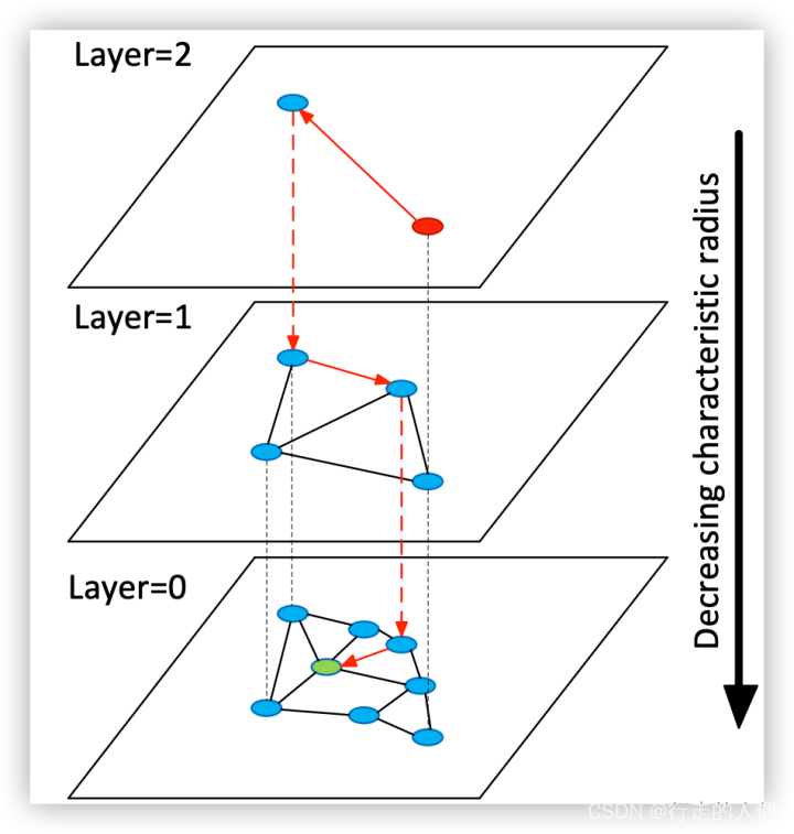

Advantage: It can find similar nearest neighbors in high-dimensional data, improving search performance. Disadvantage: Graph construction is complex, affecting memory efficiency.

3, Hash-based methods

Hash-based methods primarily exploit a property of hash functions: highly similar data have similar hash values. Hash functions can transform high-dimensional data into low-dimensional data, greatly improving index construction efficiency. However, hash functions also have another limitation: data with similar hash values are not necessarily similar, resulting in relatively low recall for this approach. 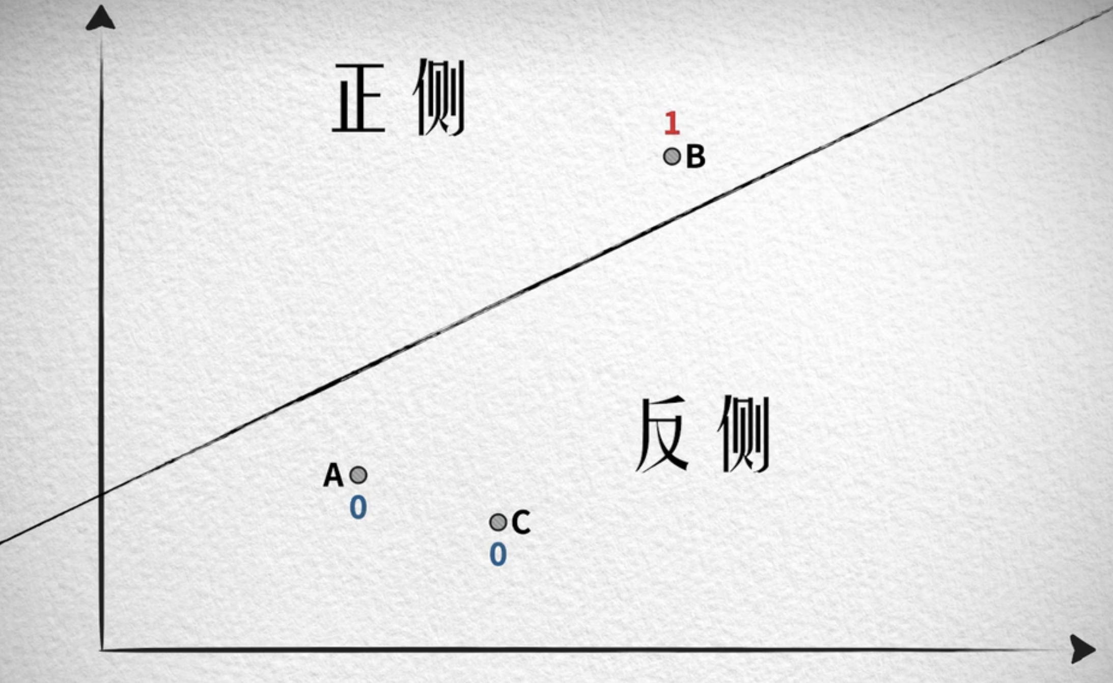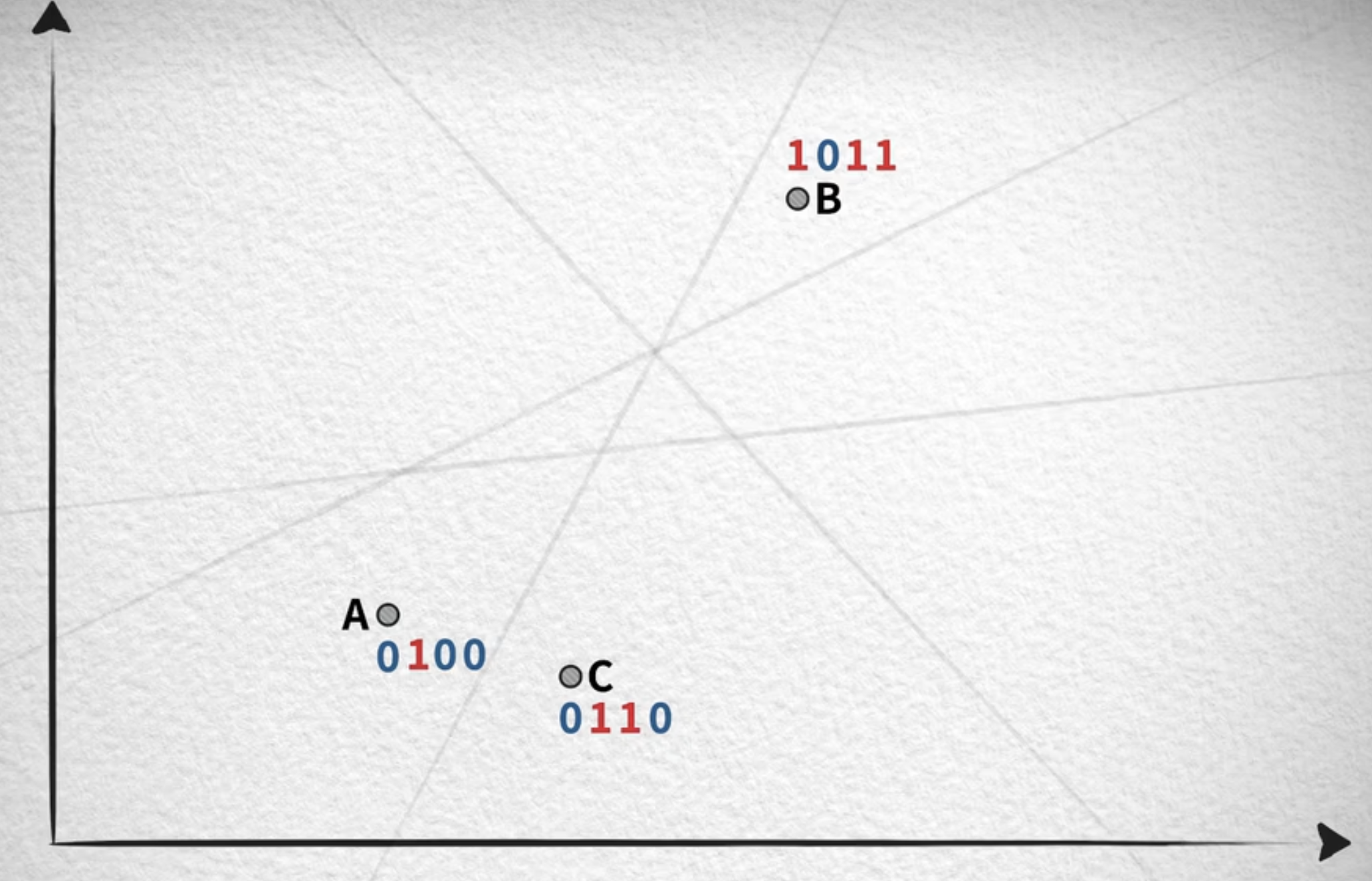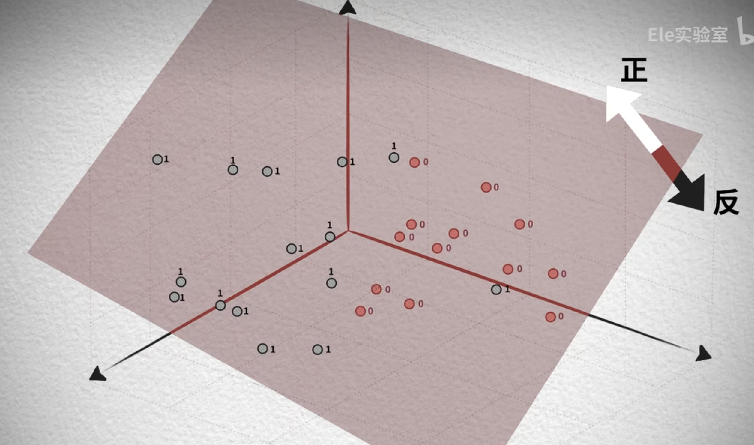The main hash-based method is LSH (Locality-Sensitive Hashing). Assuming two vectors are similar, their hash values will also be similar. A hash function maps similar vectors into the same bucket. During a query, the bucket most similar to the query vector is found first, and then the data within that bucket are searched to calculate the topk most similar results.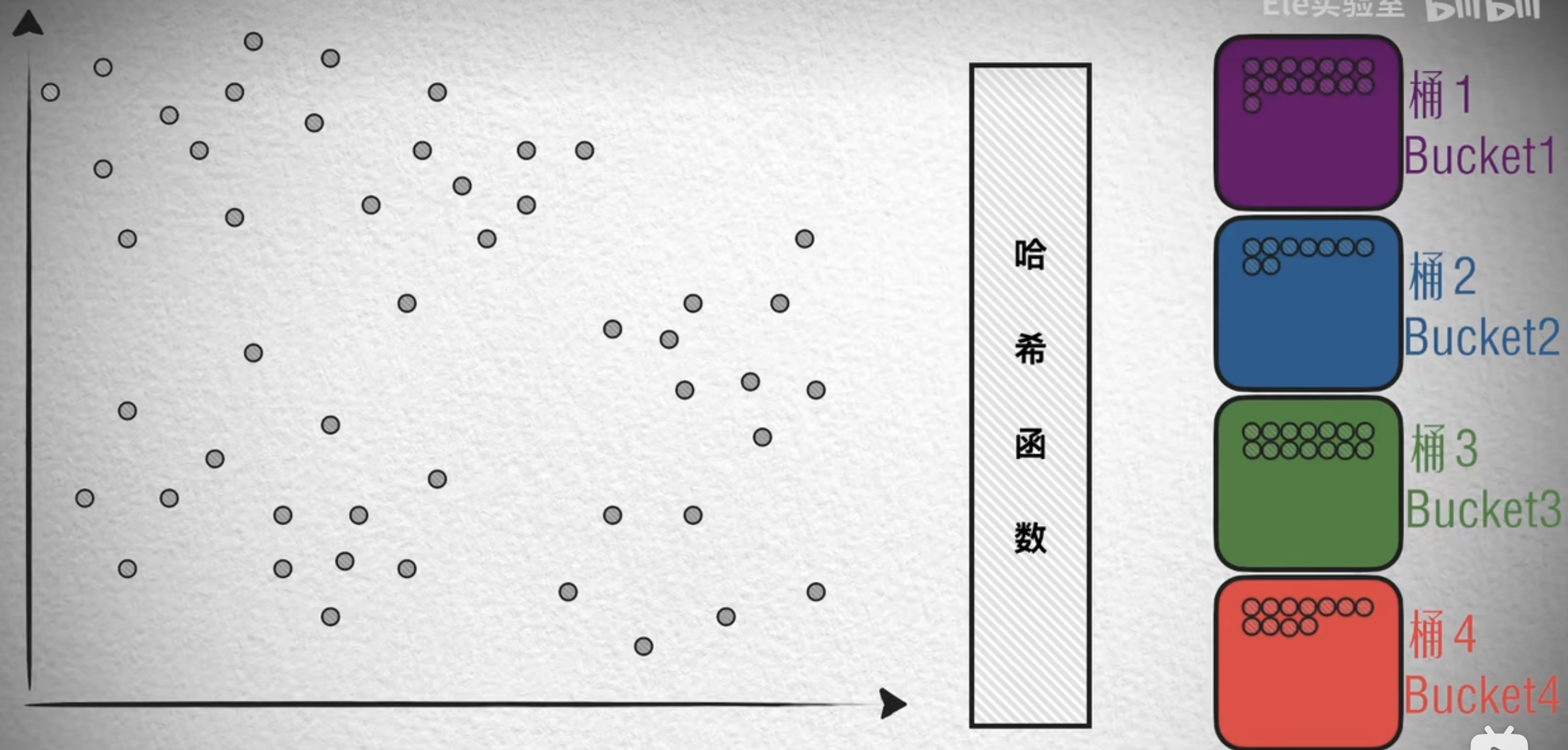
LSH (locality-sensitive hashing) is also a method based on space partitioning. Here is how it works: as shown in the diagram below, randomly generate a straight line that separates a positive side from a negative side. If a vector is on the positive side of the line, it is assigned 1; on the negative side, 0. 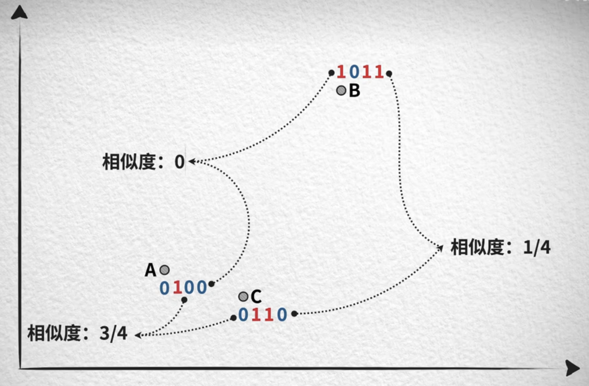Then randomly generate another straight line, again assigning 1 to the positive side and 0 to the negative side; by generating multiple such lines, we calculate 4 values of 0 or 1 for each vector, giving each a 4-bit binary code. Now let us examine how similar these 4 binary codes are.

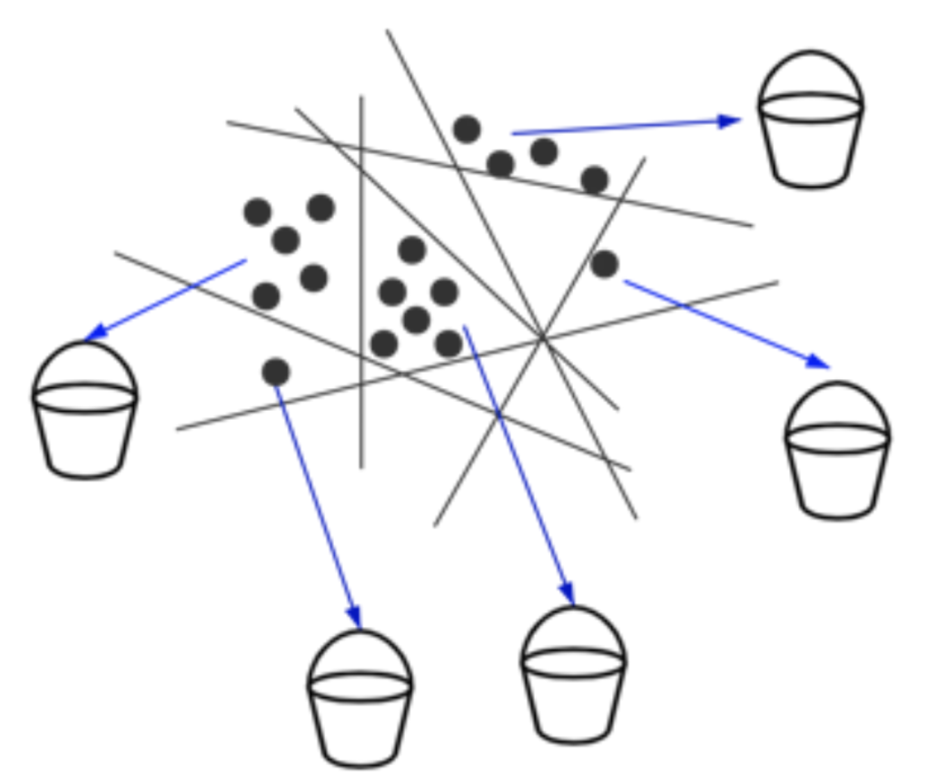
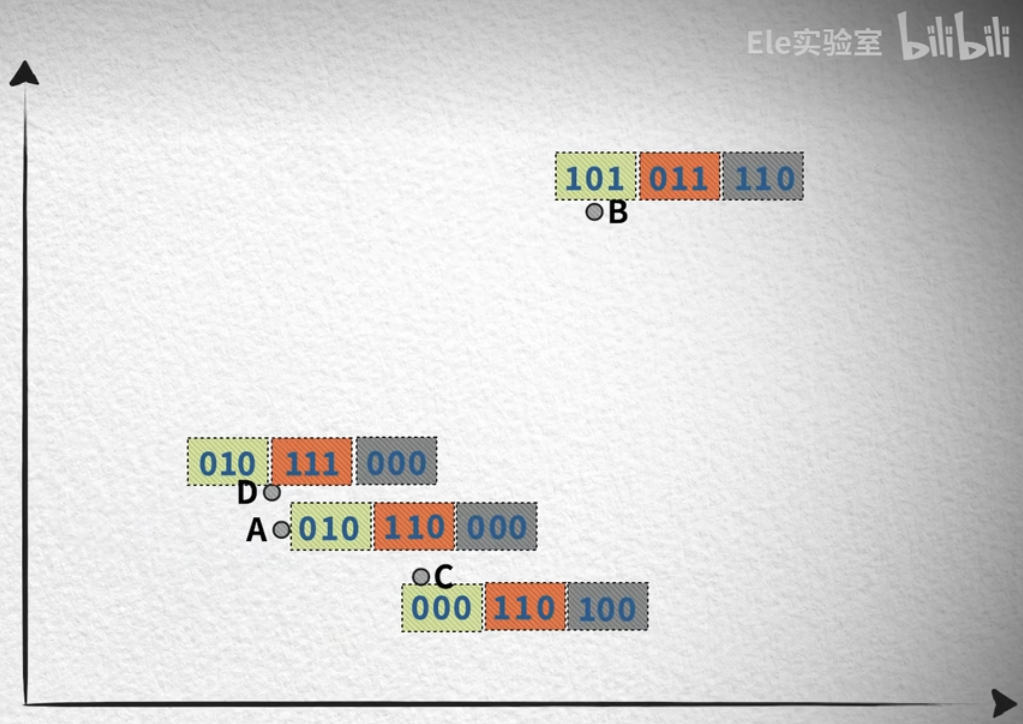
Advantage: Very fast when scaling to large datasets; disadvantage: Mediocre accuracy

5, quantization-based indexes

5.1, Clustering
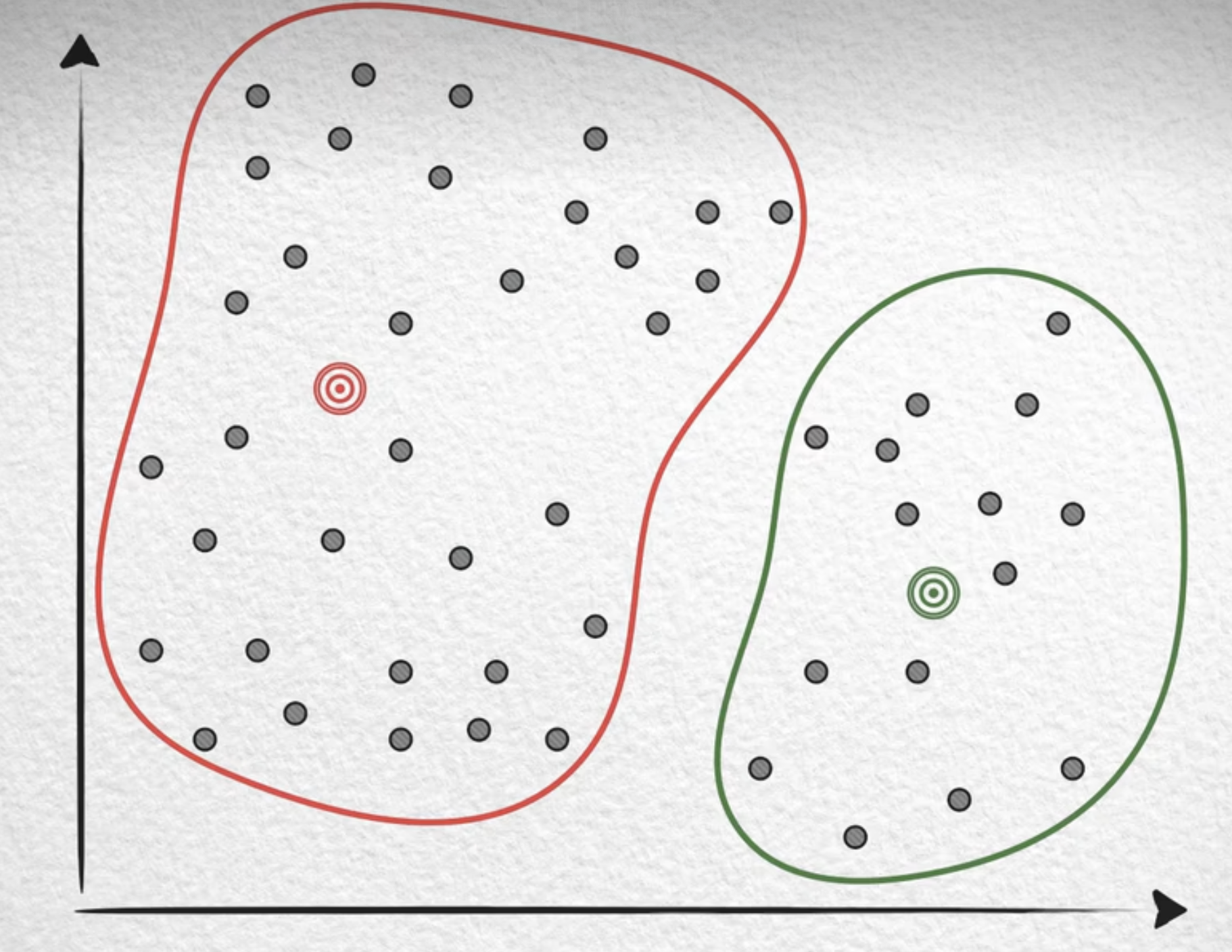
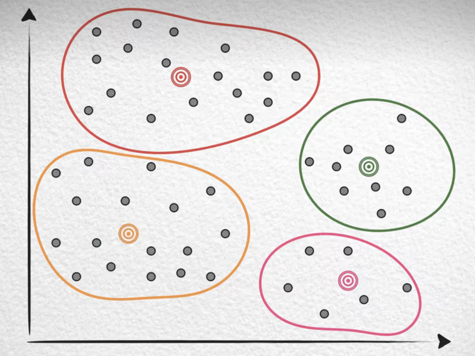
If we can define a rough search range for a query vector and then search within it, we can greatly improve search speed. First, we choose the desired number of clusters, such as the 4 clusters in the figure below, and randomly generate 4 center points. Each vector is then assigned to whichever center point is closest. Next, we calculate a mean vector from the vectors currently assigned to each cluster, move the center point to that mean vector, and then determine which center point is closest to each vector and reassign the vectors. This repeated process is called training, and eventually these center points will become stable, or converge. During a search, we only need to find the cluster center closest to the query vector and search the vectors in that cluster. This achieves the goal of narrowing the search range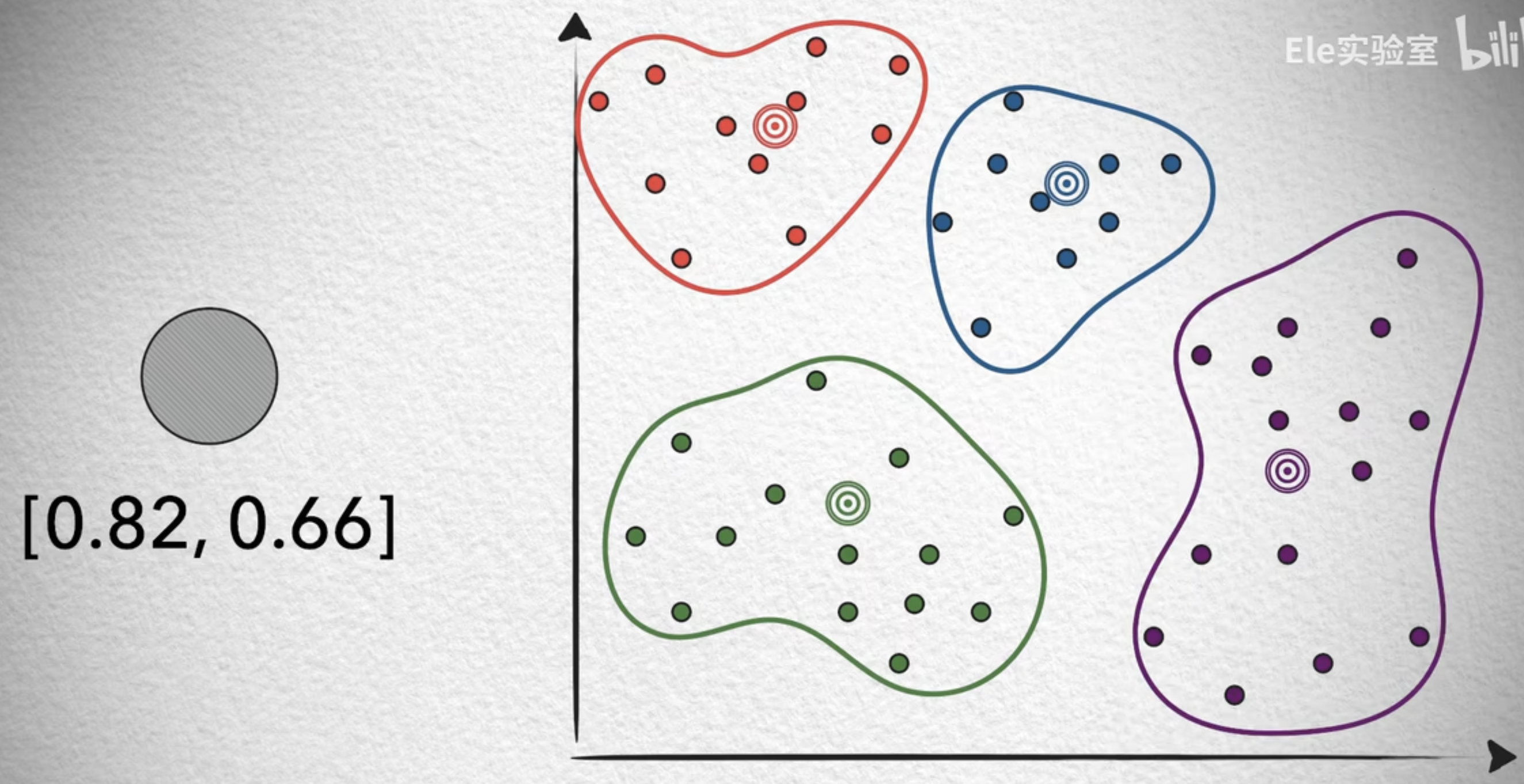

5.2, Quantization
But with massive amounts of vector data, memory overhead is another enormous challenge besides search speed. In real applications, vectors with thousands of dimensions and datasets containing hundreds of millions of vectors are not uncommon, so memory overhead can be substantial.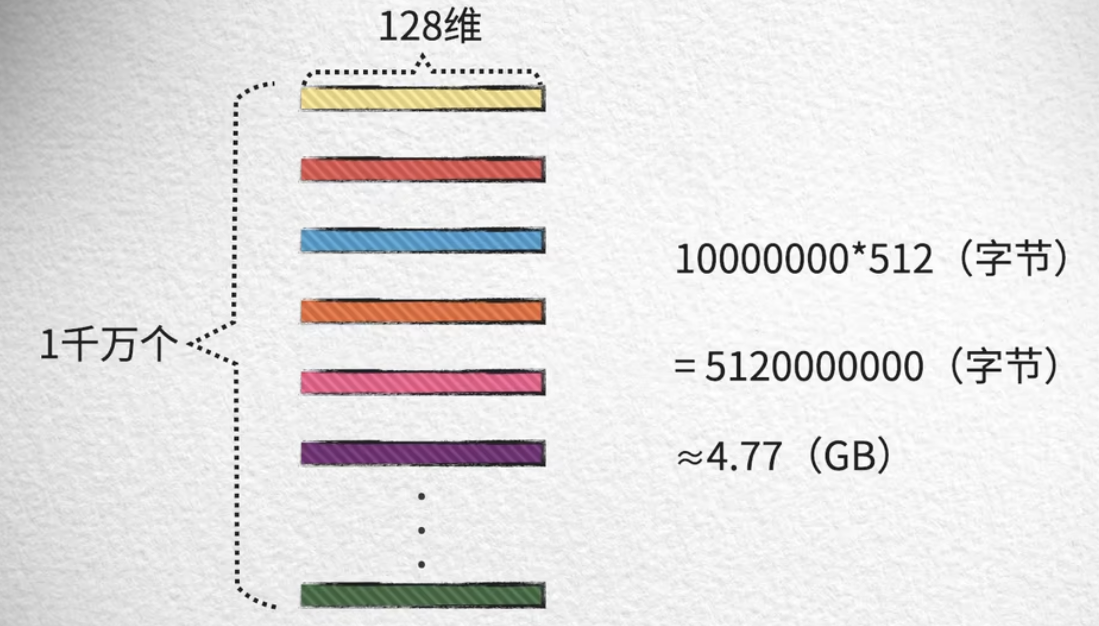

From the clustering above, we learned about the center point, which is actually called the centroid. Can we use the centroid to represent the points in a cluster? We should be able to. In fact, this method is a typical example of Lossy Compression ，illustrated with an image, it looks like this: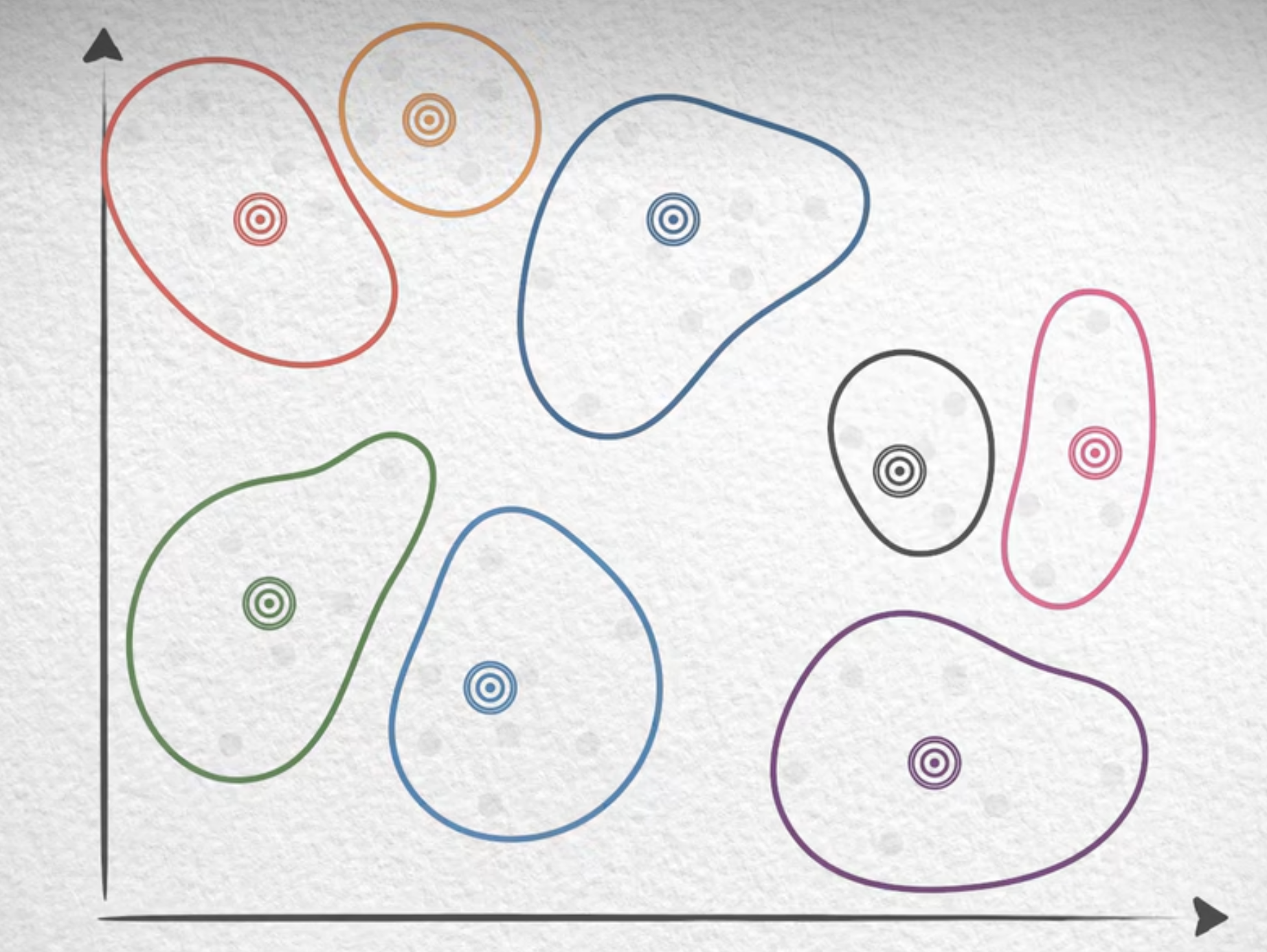

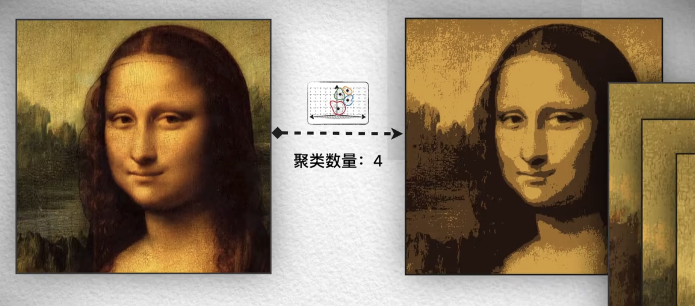
Although this loses some vector values, the correlation between a cluster centroid and the vectors in its cluster means that much of the original information is preserved. The benefits are considerable compared with the loss of some detail caused by this lossy compression. Storage can follow the diagram below: when a vector is needed, use its code to find the corresponding centroid in the codebook, then reconstruct the centroid's specific values. Representing vectors using centroid codes is what is known as vector quantization (Quantization)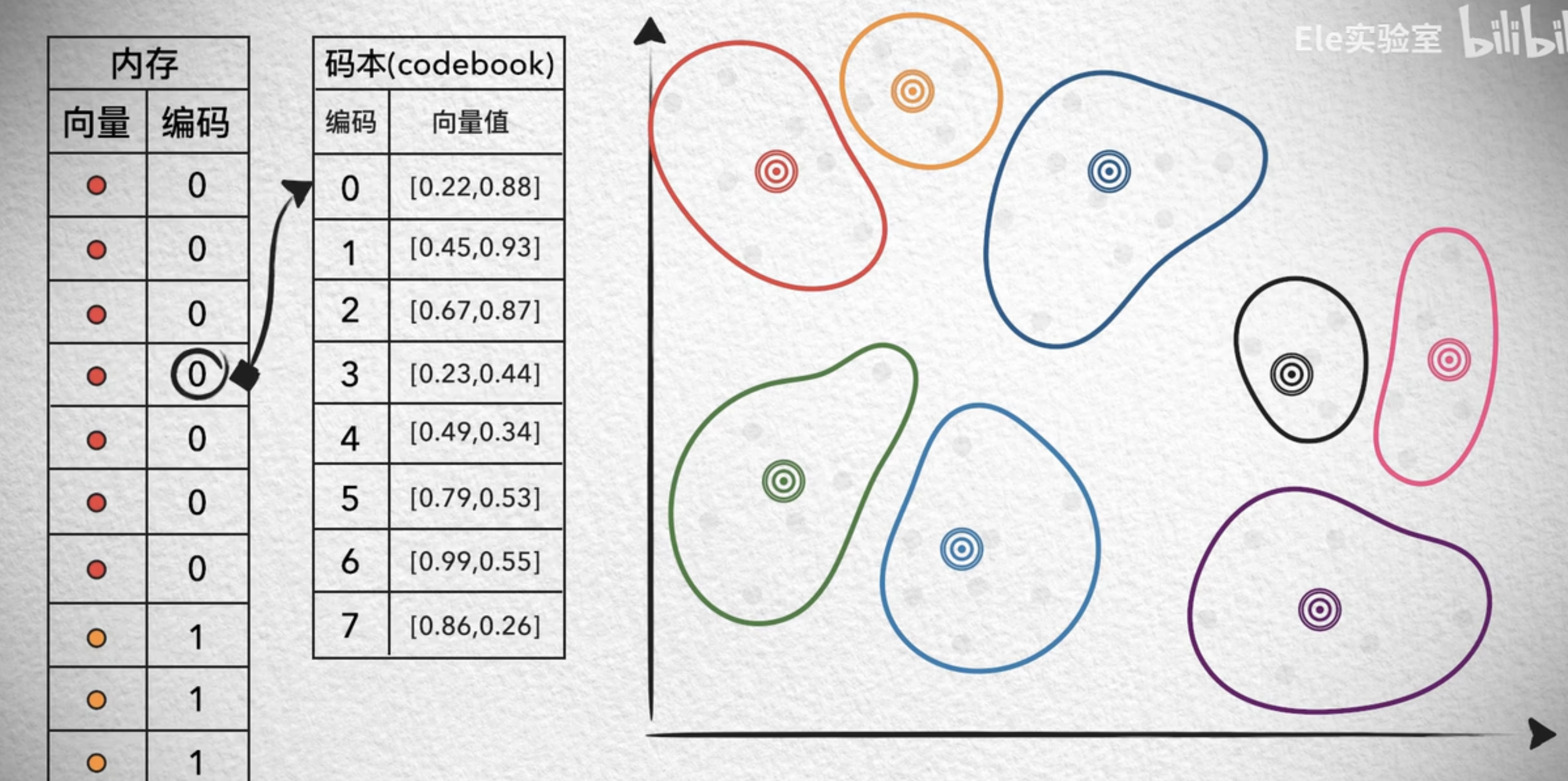

5.3, Product Quantization (PQ)
Vector quantization introduces a codebook. Although the memory overhead of the vectors themselves certainly decreases, this codebook creates additional memory overhead, and a substantial amount at that. This is less noticeable at low dimensions, but with the hundreds or thousands of vector dimensions found in real-world scenarios, the codebook can become alarmingly large. For a fixed number of vectors, maintaining quantization quality requires more cluster vectors as the vector distribution becomes sparser.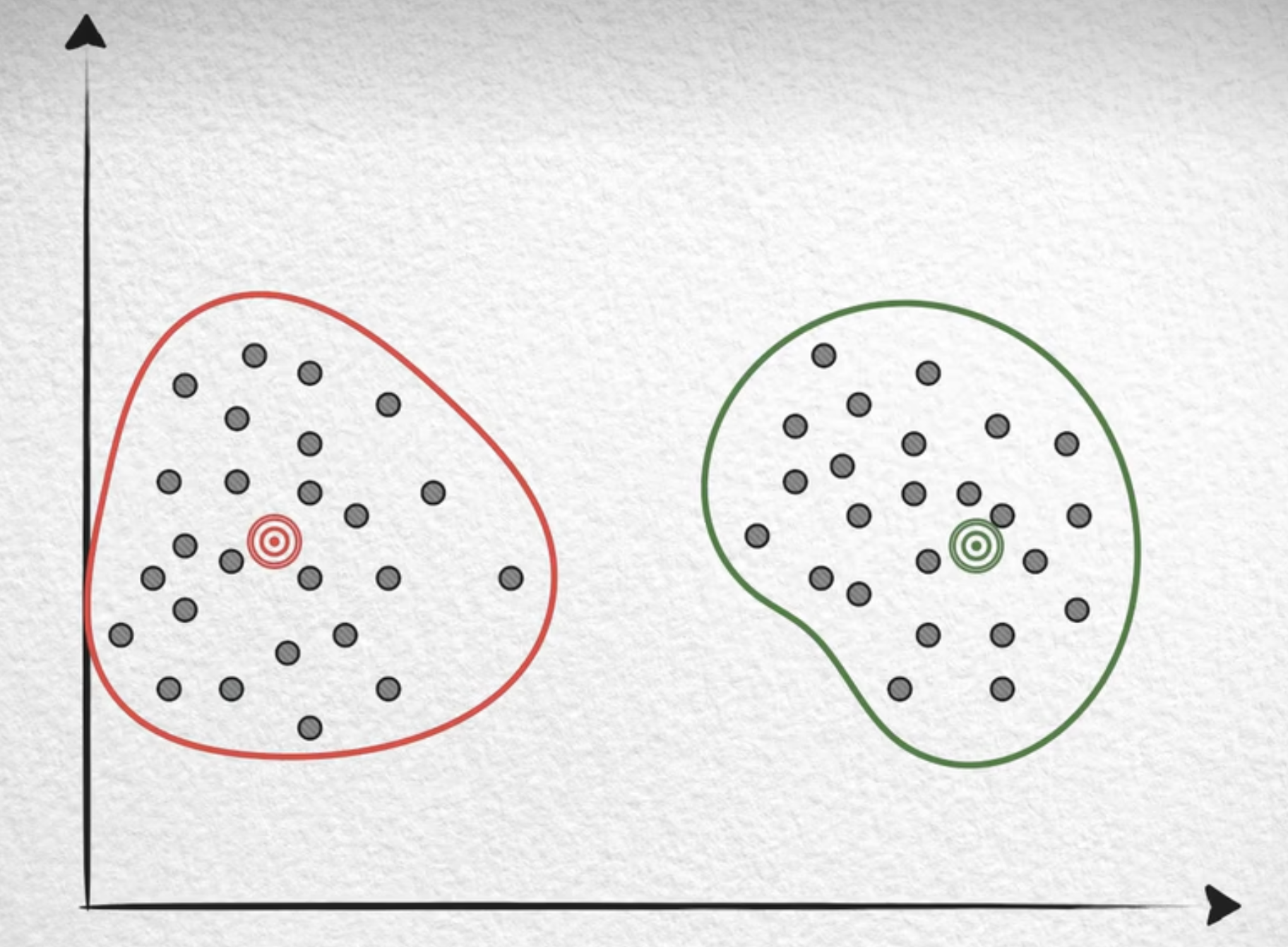

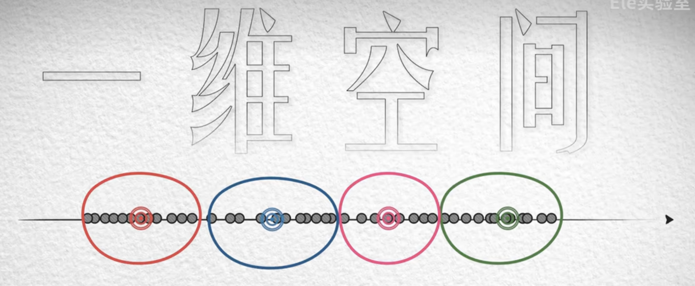
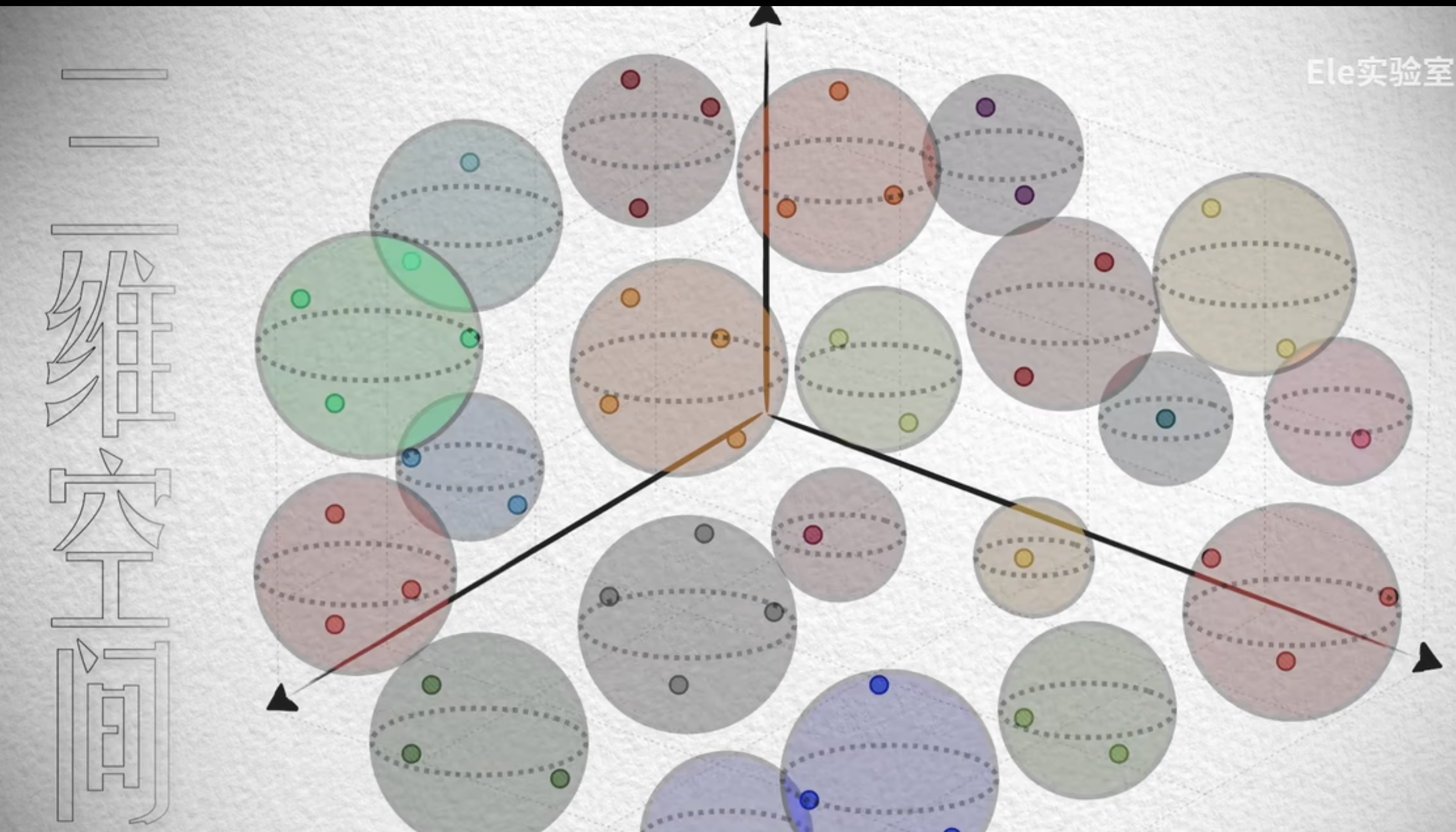
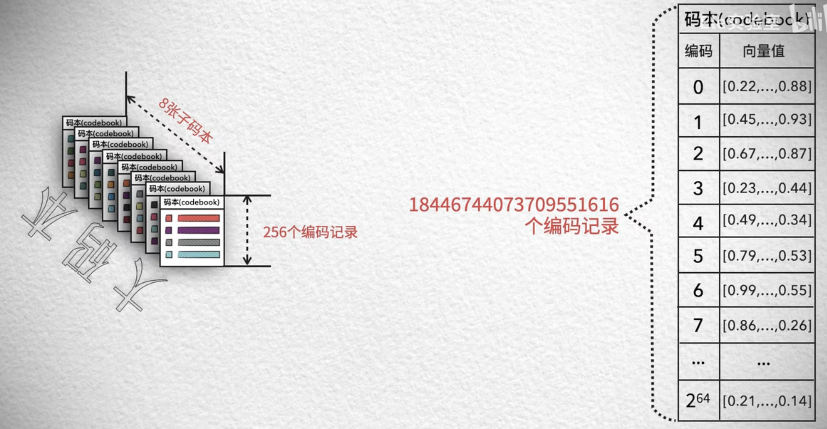
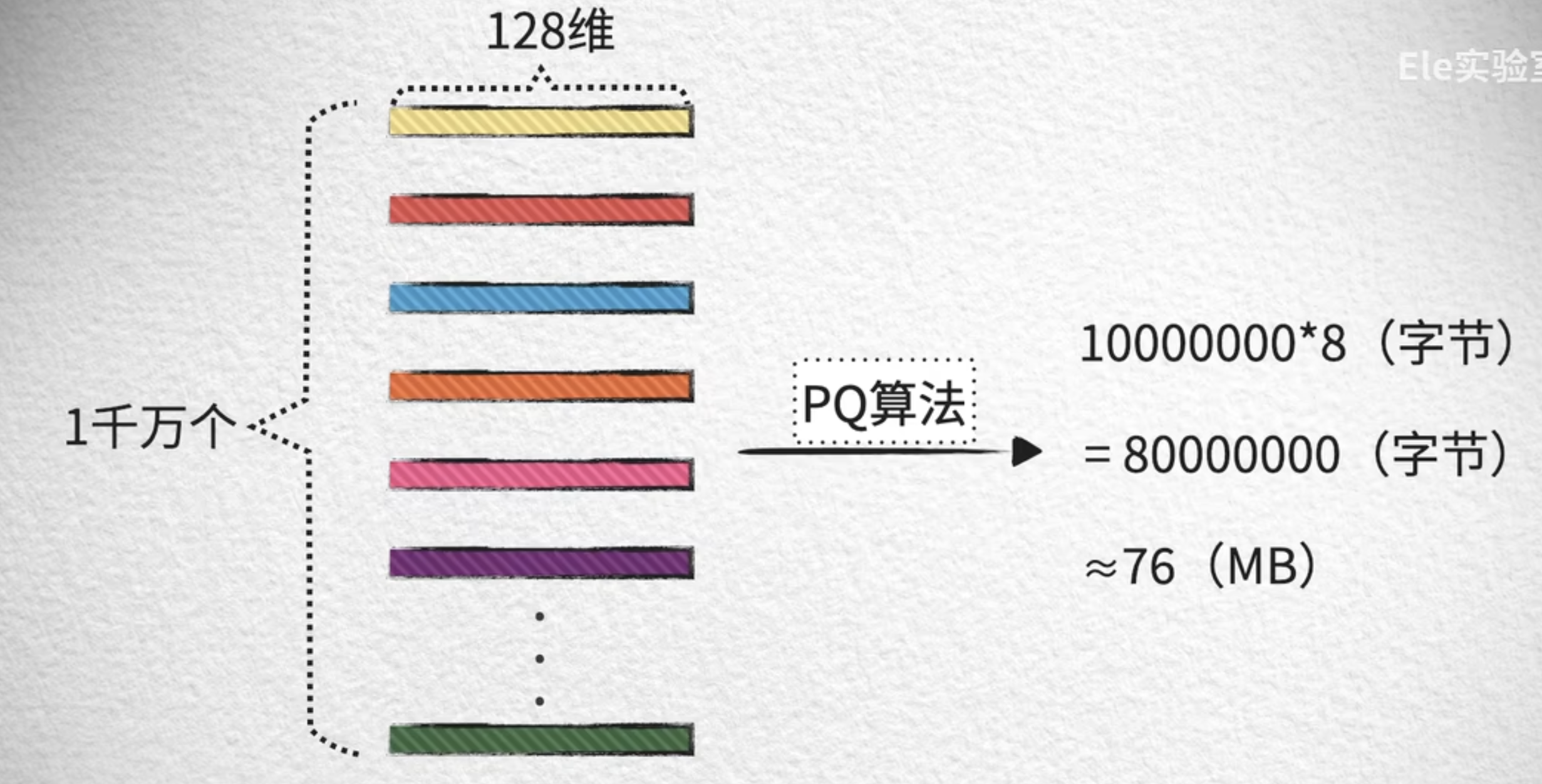
With the hundreds or thousands of vector dimensions found in real applications, data becomes extremely sparse. To ensure quantization quality in high-dimensional spaces, we may therefore need an enormous number of clusters. A typical case is shown below: a 128-dimensional vector may require 2 to the power of 64 cluster centers, which makes the codebook used to record centroid encodings enormous. The memory consumed by storing this codebook already far exceeds the memory saved by quantization itself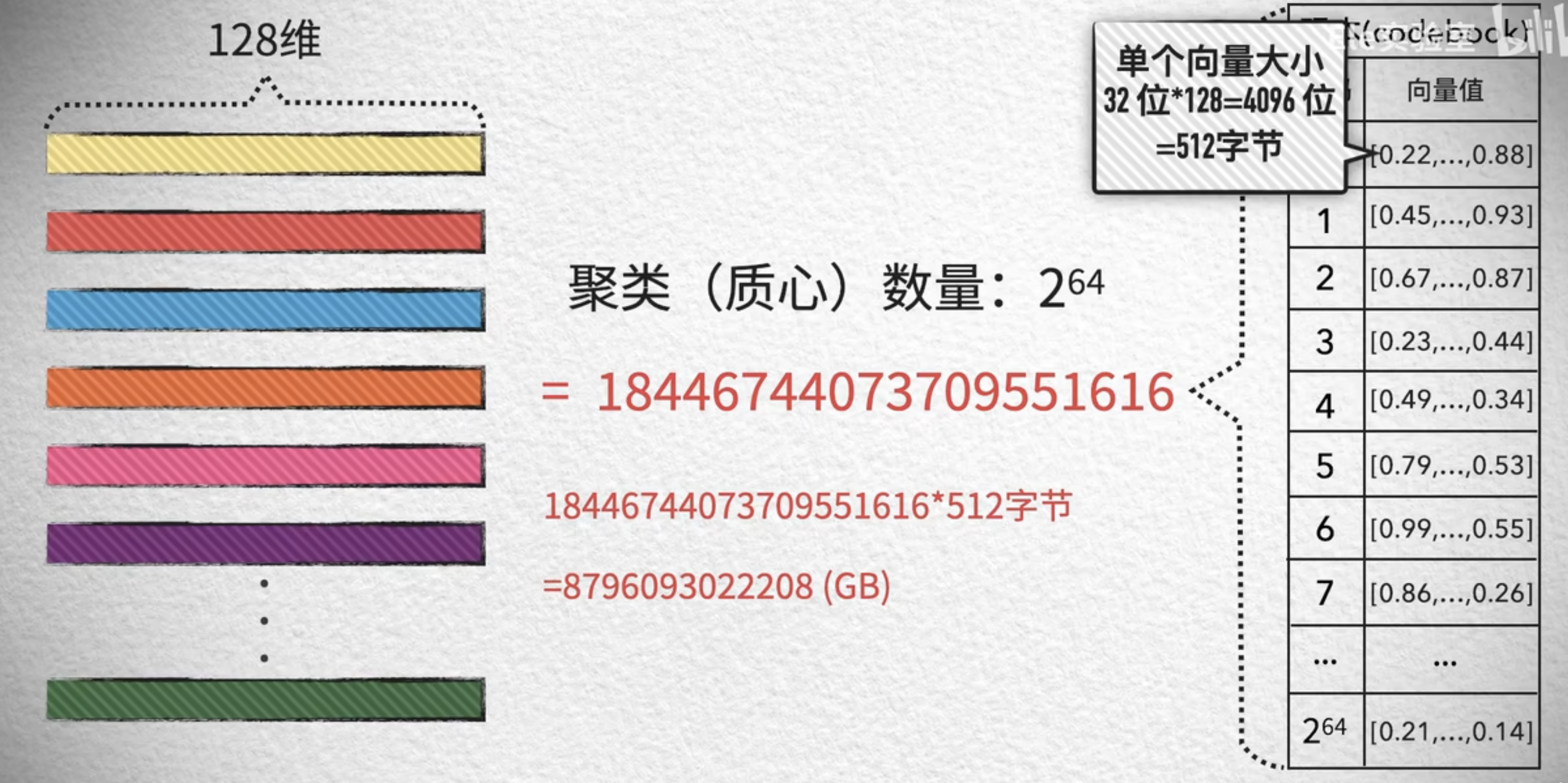
The solution is to divide the high-dimensional vector into several low-dimensional subvectors, then quantize these subvectors independently. For example, divide a 128-dimensional vector into 8 subvectors of 16 bits, then independently perform clustering training on each of the 8 16-dimensional subvectors.

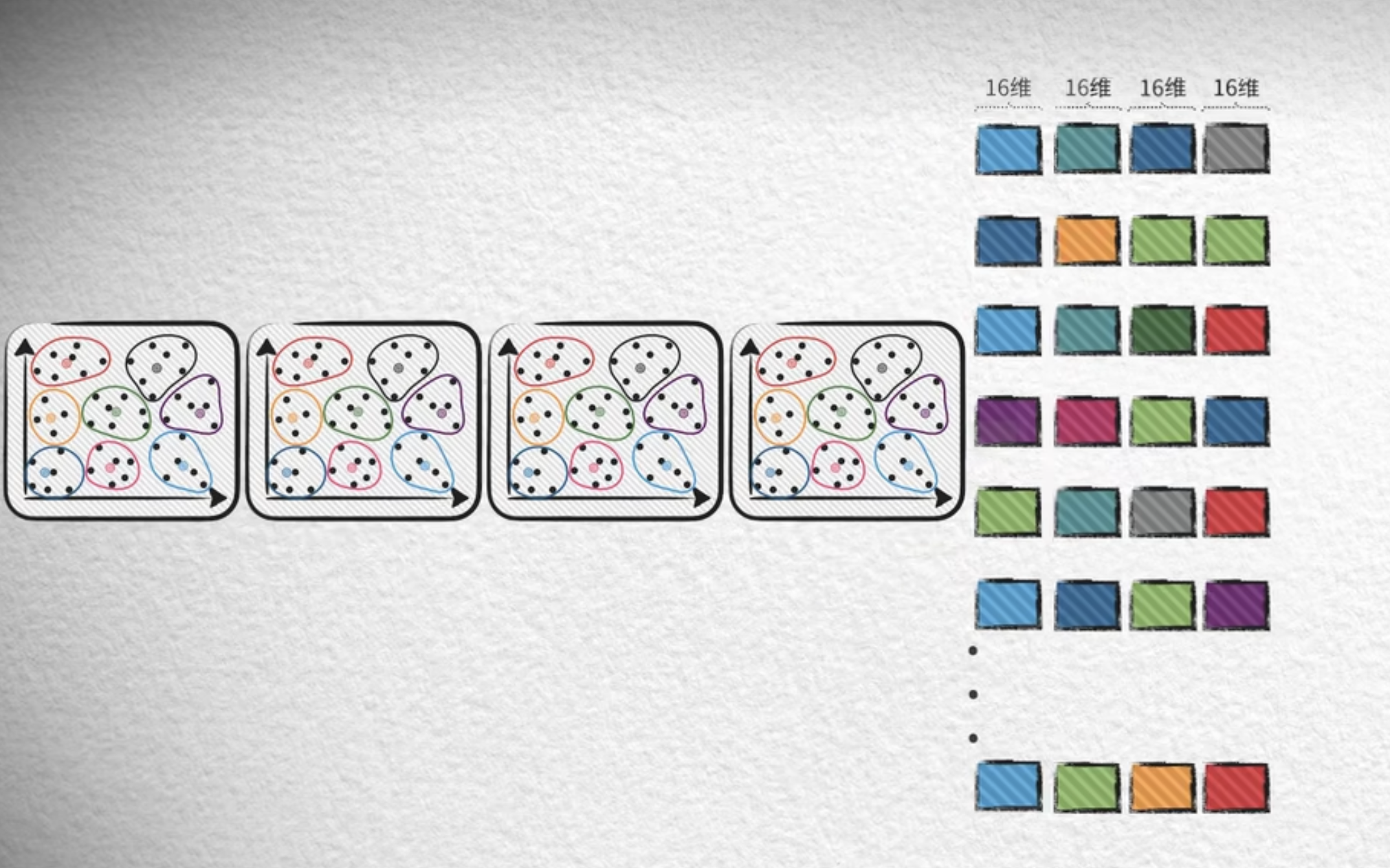
Each vector can therefore use the training results from 8 subspaces to quantize its corresponding 8 subvectors. Each subvector has 16 dimensions, which is not very high, so each 16-dimensional subspace needs only 256 clusters to achieve reasonably good quantization. Each subvector's code thus falls within the range 0-255. Combining the quantization codes of the 8 subvectors gives the final quantization code for the original vector. In other words, a vector is now quantized into 8 code values. Each subspace also builds its own sub-codebook. During use, the 8 code values are used to look up 8 subvectors of 16 dimensions in the sub-codebooks, which are then combined to reconstruct a 128-dimensional vector